Vector tiles?
When MapQuest and later Google Maps came on the scene we were blown away by the detail, speed, and convenience of “slippy maps” that you could scroll, pan, and drag across. The concept underpinning those maps was the use of tiles: pre-rendered map cells for every specified zoom level that would be loaded by your browser as you scrolled through a map. For many years after their introduction, these slippy maps used raster-based bitmaps as their tiles. As these tiles were images, that the only information available was pixel and colour.
R packages like ggmap can retrieve raster-based tiles to use as backgrounds for ggplot maps. Even if using raster tiles from different providers offering different styles (e.g. Stamen or Thunderforest or OSM), in the end the user was resigned to essentially having an unalterable image in their plot with no control over what exactly is displayed in those features.
Unlike raster tiles, vector tiles are just layers of numbers and strings containing geometry and metadata. Because they use far less data to transfer, vector tile based maps are much faster and more responsive, and most map services now use them instead. Google Maps has been vector tile based for over 5 years now.
In this simple demo, I want to focus on the advantages that come with using vector tiles. The metadata embedded within vector tile objects is what provides information on what those objects are such as type and name–and that allows a lot of flexibility in choosing what is useful and what is not.
Mapzen and rmapzen
This post relies on Tarak Shah’s excellent rmapzen package which provides an R front-end to several Mapzen APIs. From the description:
rmapzen is a client for any implementation of the Mapzen API. Though Mapzen itself has gone out of business, rmapzen can be set up to work with any provider who hosts Mapzen’s open-source software, including geocode.earth, Nextzen, and NYC GeoSearch from NYC Planning Labs. For more information, see https://mapzen.com/documentation/. The project is available on github as well as CRAN.
Mapzen was an innovative business that tried to be viable by making unreal open-source software with an emphasis on web mapping and geography products. These tools included a digital map rendering engine, search and routing services, open-source data tools for map data, terrain, and transit, gazetteers, and tile servers. This included an excellent vector tile service using OpenStreetMap data. Unfortunately Mapzen is now defunct but a number of other providers continue to host Mapzen’s open-source tools.
Thanks to an AWS Research Award Nextzen will continue to host the vector tile service through 2018 (and hopefully longer).
Install and get yourself an API key
install.packages("rmapzen")
library(rmapzen)
Create a key at (https://developers.nextzen.org) and save it as an environment variable or as an option in your .rprofile for persistence across sessions, and tell rmapzen to use Nextzen as it’s tile host. (The package author has developed interfaces to a few other hosting services since Mapzen shutdown.)
options(nextzen_API_key="your_key")
mz_set_tile_host_nextzen(key = getOption("nextzen_API_key"))
An example
In this example I will use spatial data for cities in the Victoria, British Columbia area and I wanted to add detailed vector tile base maps to improve the maps.
Some spatial data
This will work with any kind of spatial data but for convenience sake I will use Census polygons data for population from the cancensus package.
library(cancensus)
victoria <- get_census(dataset='CA16',
                       regions=list(CSD=c("5917034","5917040","5917021","5917030","5917041","5917047")),
                       vectors=c(), labels="detailed", geo_format='sf', level='CT')
And here’s what that data looks like with a little bit of styling on top:
library(ggplot2)
ggplot(victoria) +
geom_sf(aes(fill = Population)) +
scale_fill_viridis_c() +
guides(fill = guide_legend()) +
coord_sf(datum = NA) +
theme_void()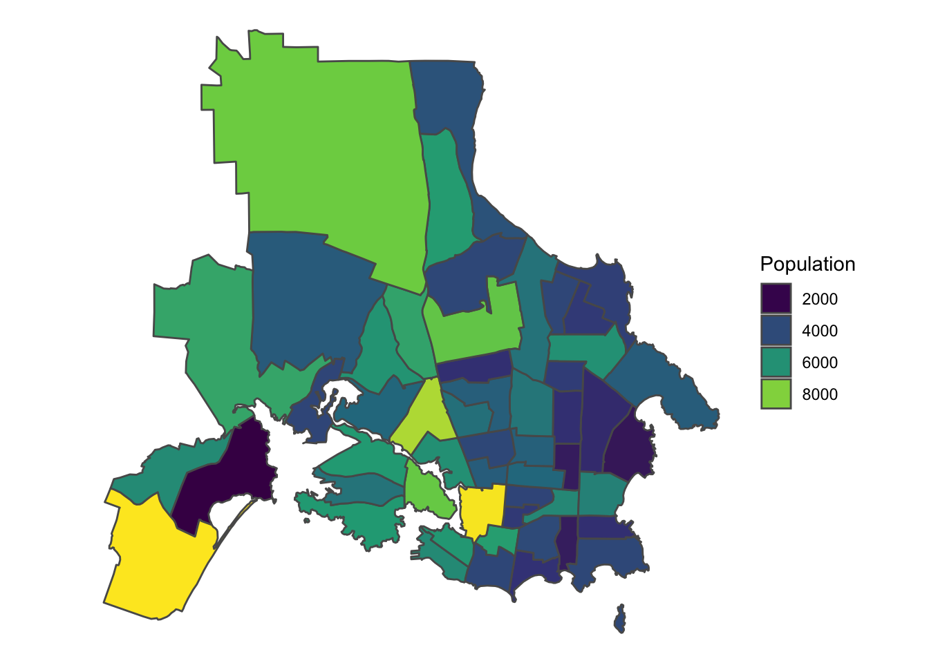 Not bad, but it’s missing the contextual geography and additional detail that comes with basemaps.
Adding vector tiles
You can download tiles by specifying bounding box of coordinates. There’s a few ways of doing this, but I find with my workflow I will typically start off with some existing spatial data for which I want to have a vector tile-based background. To that end, I use the boundary extents of my spatial data of interest to create an appropriate bounding box for my download. There’s a custom function I wrote that helps me with this:
get_vector_tiles <- function(bbox){
  mz_box=mz_rect(bbox$xmin,bbox$ymin,bbox$xmax,bbox$ymax)
  mz_vector_tiles(mz_box)
  }
Which I then combine with a call to st_bbox from the sf package to grab vector tiles.
library(sf)
bbox <- st_bbox(victoria)
vector_tiles <- get_vector_tiles(bbox)
The vector_tiles object is a list of spatial feature layers. Depending on what information is available for the selected geographic area there may be more or fewer layers. In this case, this set of vector tiles has 9 layers, though sometimes these layers are empty despite being downloaded so it’s worth checking.
names(vector_tiles)## [1] "water" "buildings" "places" "transit" "pois"
## [6] "boundaries" "roads" "earth" "landuse"# check if this layer has no data
vector_tiles$transit## Mapzen vector tile layer
## No dataHaving each of these as separate layers gives us a lot of flexibility in designing our maps because we can turn each layer into its own object, control the order of rendering, and style it however we want–or choose to exclude them altogether. We can also turn these layers into sf or sp objects and do any spatial analysis or manipulation that you can do with other spatial objects. In this case, I want to keep the water and theroads layers for my map.
water <- as_sf(vector_tiles$water)
roads <- as_sf(vector_tiles$roads)
We can take a look at what these objects look like visually.
ggplot(roads) +
geom_sf() +
theme_void() +
coord_sf(datum = NA)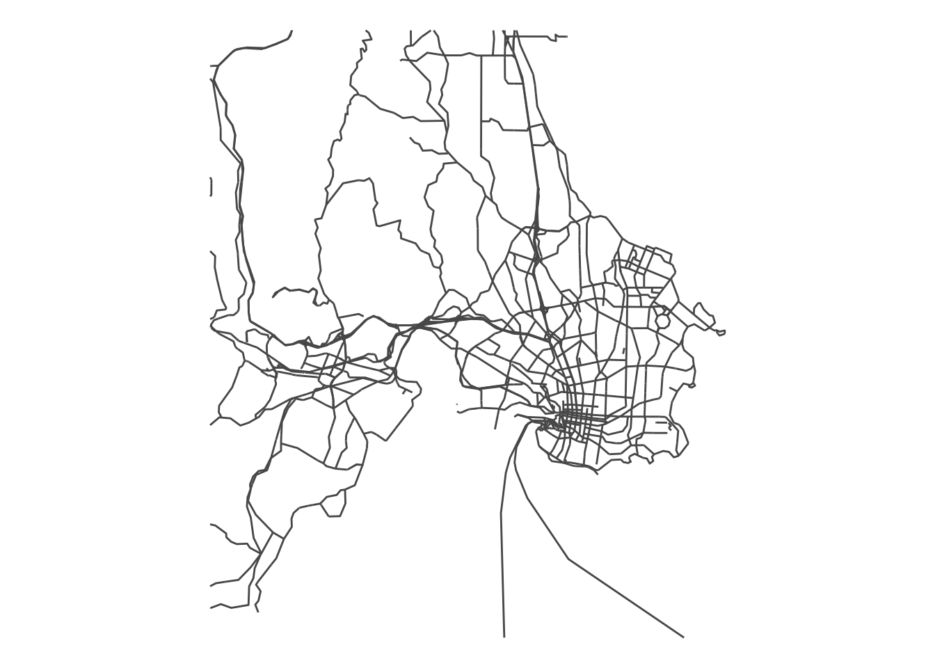 Clearly the
 roads layer includes much more than roads alone. It’s collection of features with many different fields for each object that tell us more about what those roads actually are, and allow us to have that much more control over representing these objects still.
names(roads)## [1] "kind" "sort_rank" "kind_detail"
## [4] "is_bicycle_related" "surface" "bicycle_network"
## [7] "source" "min_zoom" "bicycle_shield_text"
## [10] "id" "name" "bus_network"
## [13] "cycleway" "bus_shield_text" "landuse_kind"
## [16] "is_link" "walking_shield_text" "walking_network"
## [19] "all_networks" "shield_text" "ref"
## [22] "all_shield_texts" "network" "loc_name"
## [25] "cycleway_right" "cycleway_left" "name.en"
## [28] "name.fr" "access" "geometry"We can look at what kind of data each of those elements has.
table(roads$kind)##
## ferry highway major_road minor_road path rail
## 5 38 775 22 47 7table(roads$cycleway)##
## lane shared shared_lane track
## 203 10 5 2table(roads$surface)##
## asphalt compacted concrete gravel paved
## 100 11 2 7 118
## paving_stones unpaved wood
## 1 3 5With this information in hand we can split the roads object into different components representing different types of “roads”. The information
library(dplyr)##
## Attaching package: 'dplyr'## The following objects are masked from 'package:stats':
##
## filter, lag## The following objects are masked from 'package:base':
##
## intersect, setdiff, setequal, unionggplot() +
geom_sf(data = roads %>% filter(kind == "ferry"), colour = "red") +
geom_sf(data = roads %>% filter(kind == "highway"), colour = "blue") +
geom_sf(data = roads %>% filter(kind == "rail"), colour = "green") +
geom_sf(data = roads %>% filter(kind == "major_road"), colour = "darkgrey") +
geom_sf(data = roads %>% filter(cycleway == "lane"), colour = "orange") +
theme_void() +
coord_sf(datum = NA)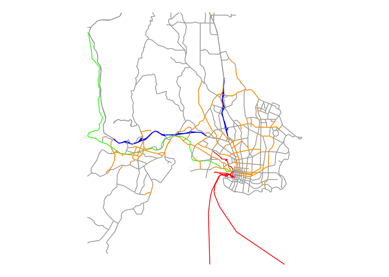
More control over your maps
Putting aside their obvious use for interesting spatial analysis and data, vector tiles give you an enormous amount of flexibility for designing maps by allowing you to customize the styling of each component individually if you were inclined to do that. The end result means that you can take something that looks like this:
ggplot(victoria) +
  geom_sf(aes(fill = Population)) +
  scale_fill_viridis_c() +
  guides(fill = guide_legend()) +
  coord_sf(datum = NA) +
  theme_void()
And improve it with vector tiles so it looks like this:
ggplot(victoria) +
geom_sf(aes(fill = Population), colour = NA) +
geom_sf(data = water %>% filter(kind %in% c("ocean", "lake", "river")), fill = "lightblue") +
geom_sf(data = roads %>% filter(kind == "ferry"), colour = "grey90", size = 0.5) +
geom_sf(data = roads %>% filter(kind == "highway"), colour = "grey10", size = 1.25) +
geom_sf(data = roads %>% filter(kind == "rail"), colour = "brown") +
geom_sf(data = roads %>% filter(kind == "major_road"), colour = "grey20") +
geom_sf(data = roads %>% filter(cycleway == "lane"), colour = "grey30") +
scale_fill_viridis_c() +
guides(fill = guide_legend()) +
coord_sf(datum = NA) +
theme_void()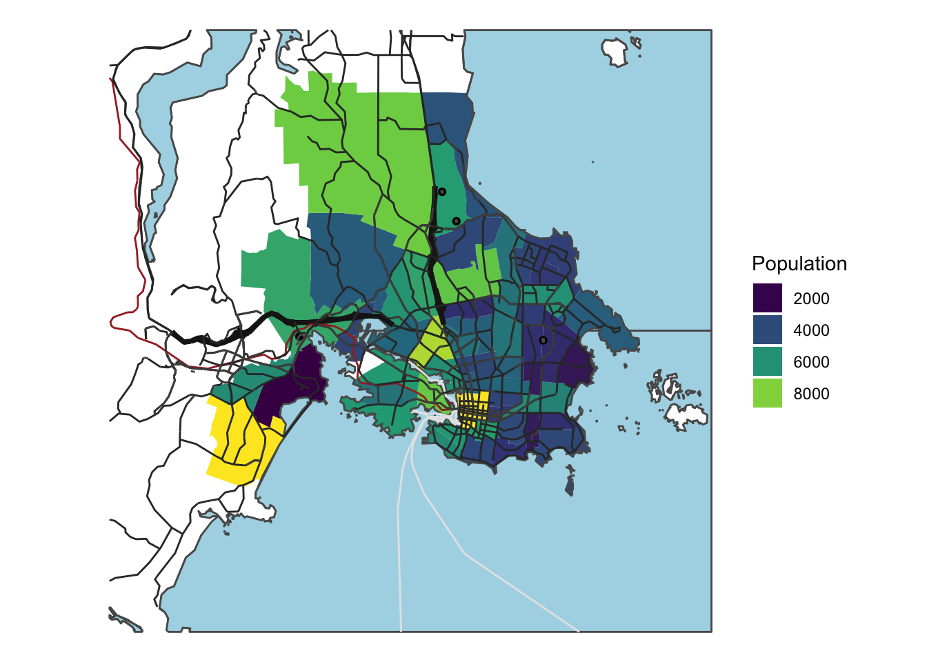 And sometimes the additional geographic contextual information from vector tiles can go a long ways in explaining data presented on a map. Consider the following plot of logged population density in Vancouver, Burnaby, and New Westminster cities in the Metro Vancouver region.
 A dense downtown peninsula is clear, but the diagonal swathe of density across the city of Vancouver would only immediately make sense to someone familiar with the area who would recognize that the density reflects the shape of the Skytrain rapid transit network.
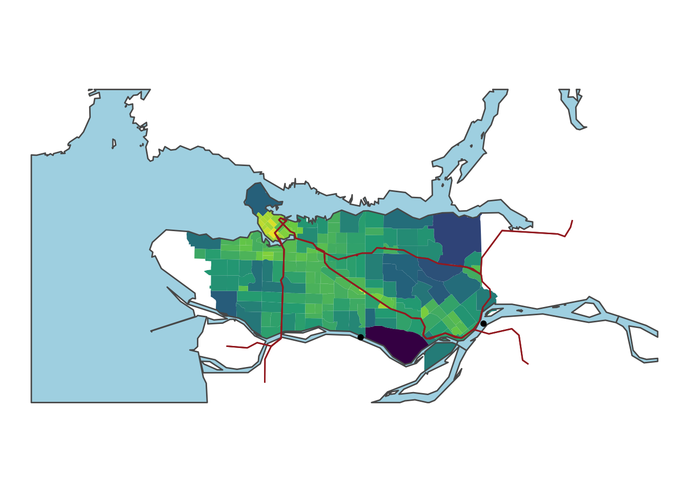 It’s worth it to invest the time to add a bit more style and a lot more contextual information to your maps by using vector tiles.
Can’t I just download the shape files I need?
Sure, but for something like the plot of Victoria earlier in the post you would have needed to download separate files for landmass, roads, rail, each from potentially different data sources and then would have had to clip them to meet the extent of your target data. Vector tiles have all of that in one place and can be automatically clipped to the exact areas you are working with and the required code to do all of this is pretty straightforward thanks to the excellent rmapzen package. Another advantage is built-in object simplification: most maps will work just fine with simplified polygons–they do not need to be at the resource survey-level accuracy that public sector shape files are typically at.
Alternative sources for vector tiles
I continue to use Nextzen for vector tiles and have no issues with usage through my free-level API access, but there are some alternatives out there like Thunderforest and Mapcat that have free/hobbyist access tiers to their vector tile APIs. There is also OpenMapTiles where you can download different types of vector tiles in bulk (note that the files are enormous in size) for free for non-commercial uses.
Package info
sessionInfo()## R version 3.5.1 (2018-07-02)
## Platform: x86_64-apple-darwin15.6.0 (64-bit)
## Running under: macOS High Sierra 10.13.4
##
## Matrix products: default
## BLAS: /Library/Frameworks/R.framework/Versions/3.5/Resources/lib/libRblas.0.dylib
## LAPACK: /Library/Frameworks/R.framework/Versions/3.5/Resources/lib/libRlapack.dylib
##
## locale:
## [1] en_CA.UTF-8/en_CA.UTF-8/en_CA.UTF-8/C/en_CA.UTF-8/en_CA.UTF-8
##
## attached base packages:
## [1] stats graphics grDevices utils datasets methods base
##
## other attached packages:
## [1] dplyr_0.7.6 sf_0.6-3 ggplot2_3.0.0 bindrcpp_0.2.2
## [5] cancensus_0.1.7 rmapzen_0.3.5
##
## loaded via a namespace (and not attached):
## [1] tidyselect_0.2.4 xfun_0.3 purrr_0.2.5
## [4] lattice_0.20-35 V8_1.5 colorspace_1.3-2
## [7] htmltools_0.3.6 viridisLite_0.3.0 yaml_2.1.19
## [10] rlang_0.2.1 e1071_1.6-8 pillar_1.3.0
## [13] foreign_0.8-70 glue_1.3.0 withr_2.1.2
## [16] DBI_1.0.0 sp_1.3-1 bindr_0.1.1
## [19] plyr_1.8.4 stringr_1.3.1 geojsonio_0.6.0
## [22] rgeos_0.3-28 munsell_0.5.0 blogdown_0.8
## [25] gtable_0.2.0 evaluate_0.11 labeling_0.3
## [28] knitr_1.20 maptools_0.9-2 curl_3.2
## [31] class_7.3-14 Rcpp_0.12.17 scales_0.5.0
## [34] backports_1.1.2 classInt_0.2-3 jsonlite_1.5
## [37] digest_0.6.15 stringi_1.2.4 bookdown_0.7
## [40] grid_3.5.1 rprojroot_1.3-2 jqr_1.0.0
## [43] rgdal_1.3-3 tools_3.5.1 magrittr_1.5
## [46] lazyeval_0.2.1 geojson_0.2.0 tibble_1.4.2
## [49] crayon_1.3.4 pkgconfig_2.0.1 spData_0.2.9.0
## [52] assertthat_0.2.0 rmarkdown_1.10 httr_1.3.1
## [55] R6_2.2.2 units_0.6-0 compiler_3.5.1