What does it mean to be “normal”?
Consider for a moment the quintessential Canadian city. What does that image in your head look like? Are there outdoor rinks, wheat fields, and abundant Timmies? Does your mental image include a yoga studio, a dispensary, and a third-wave coffee shop? Canadians like to celebrate a self-constructed identity of diversity-the cultural mosaic- that is punctuated with conspicuous Canadiana that binds everything together. Canada is a highly urbanized country–it is a nation of cities, and while every Canadian city has elements that scream “Canada!”, is there a city that can stand above the rest and definitely claim to be the most quintessentially Canadian city of them all?
One way of approaching a question like this would be to define some kind of criteria that best represents this Canadian essence–but that would be hard and, truthfully, rather icky. The idea of the “normal” place is a common rhetorical approach often used to conjure up an image of a majority-dominant heartland that truly represents the values of a country. You can see this in politics all the time: cities are more diverse and heterogeneous than rural places, and, in many industrialized countries, account for the majority of the population, but are seldom viewed as representative of a country’s characteristics.
A more data-driven approach
So instead of a selecting for some arbitrary characteristics that define what the Canadian “normal” is, let’s take a data-driven approach. Fortunately, this FiveThirtyEight article by the economist Jed Kolko looking at identifying the most “normal” place in America provides a good template to start. The motivation behind the FiveThirtyEight article is simple: there is a disconnect between what pundits and some politicians view as representative of a “normal America” and what actual demographics say. The most “normal” place in America is not Oshkosh, Wisconsin but New Haven, Connecticut. Kolko’s approach is pretty simple as it relies on a quantitative analysis of demographics across US metros using age, education, and race as key indicators. The demographic mix of each metro area is compared against the demographic mix of the US as a whole using a dissimilarity index across every combination of selected demographic indicators from the American Community Survey.
We can do something similar using Canadian data. While we lack the crosstabs across Census values to apply the exact same methodology as the FiveThirtyEight article, a roughly similar approach can be taken by calculating the proportion or incidence of selected Census demographic or behavioral values for a given place and comparing it to a national benchmark. The cumulative sum of the geometric distance between the values for the national rate and that of the selected place provides an indication of similarity or dissimilarity. The most “normal” city in Canada will be the city that has the most similar demographic and characteristic makeup to the national benchmark.
The code chunk for this post is at the bottom of the page and the similarity calculations are contained in the last few lines of code.
The demographic mix
While the FiveThirtyEight article looks at age, education, and race only, we have the entire range of Canadian Census values to work with. This distinction is important because the result of any similarity calculation like the one in this post will depend on the variables that are selected. Using all available Census variables is not feasible, but we can go beyond age, education, and visible minority groups to also include immigration status, household tenure type, and commute types to capture some additional indicators that define how a city looks and feels. Income variables are not used here for several reasons: one, they are likely to be highly correlated with other variables that are included like education and household tenure; and, two, income can vary across cities, regions, and provinces for many reasons that can be specific to those places. Age and education variables are collapsed into broader groups to streamline things a bit.
Census subdivisions
Census subdivisions are a standard Statistics Canada geographic area that represents municipalities or areas deemed to be equivalent such as indigenous reserves. Using Census subdivisions instead of Census Metropolitan areas provides more granularity and more interesting results–there are some very different demographic mixes in the different cities that make up the Greater Toronto Area that could average out at the metro area. The latest Census has data for 5,148 Census subdivisions, though most of these are areas with very low population. Similarity is calculated here for the 413 subdivisions with population of 10,000 or more.
The most “normal” places in Canada
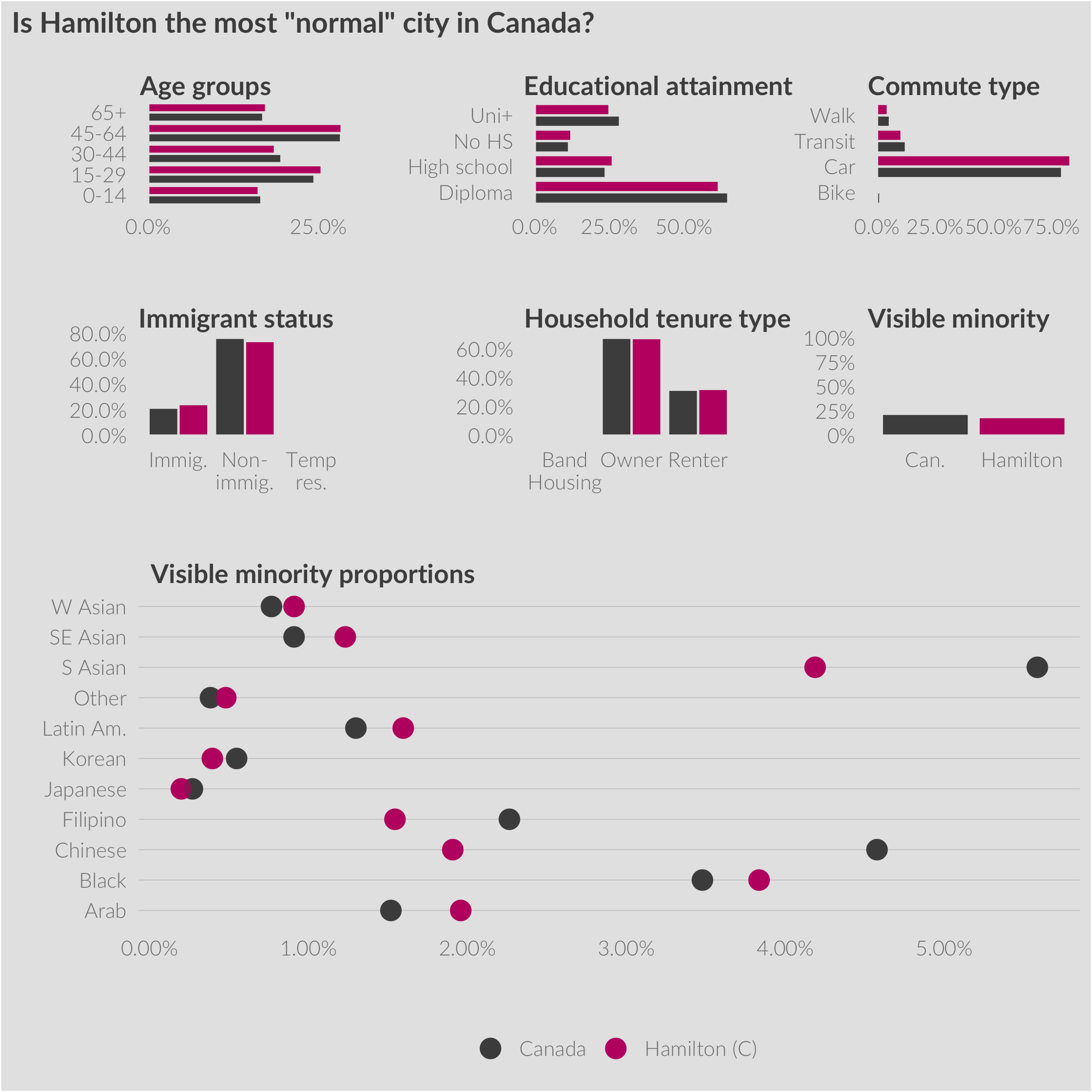
Using geometric distances between demographic and characteristic compositions the most “normal” or most representative municipality in Canada is Hamilton, Ontario. Guelph, London, Winnipeg, and Kitchener round out the bottom five.
| Municipality | Population | Similarity Score |
|---|---|---|
| Hamilton | 536,917 | 91.6 |
| Guelph | 131,794 | 89.1 |
| London | 383,822 | 88.0 |
| Winnipeg | 705,244 | 87.4 |
| Kitchener | 233,222 | 86.5 |
| Note: | ||
|
Source: Statistics Canada Census 2016. Similarity score calculated using a combination of demographic and characteristic Census variables as compared with national rates. |
Model of a modern Canadian city
 Photograph of downtown Hamilton, Ontario taken from Sam Lawrence Park, Wikipedia CC BY-SA 2.5
Hamilton has almost identical proportions to Canada as a whole for almost every variable looked at in calculating the score. Like Canada overall, the majority of the population falls into either the 45-64 or 15-29 groups that represent the Boomer and Millennial mega-generations. Educational attainment similar with the majority of people living in Canada possessing a post-secondary diploma below a university degree. The individual proportions of visible minority groups is remarkably similar as almost every group has a share of the population that falls within 1% of the national proporton.
 Compare this with the city of Vancouver, below, which drastically differs from the national averages in across all categories. Vancouver has fewer children under 15, more university educated people, a far higher incidence of renters and immigrants, and a far lower incidence of commuting by car.
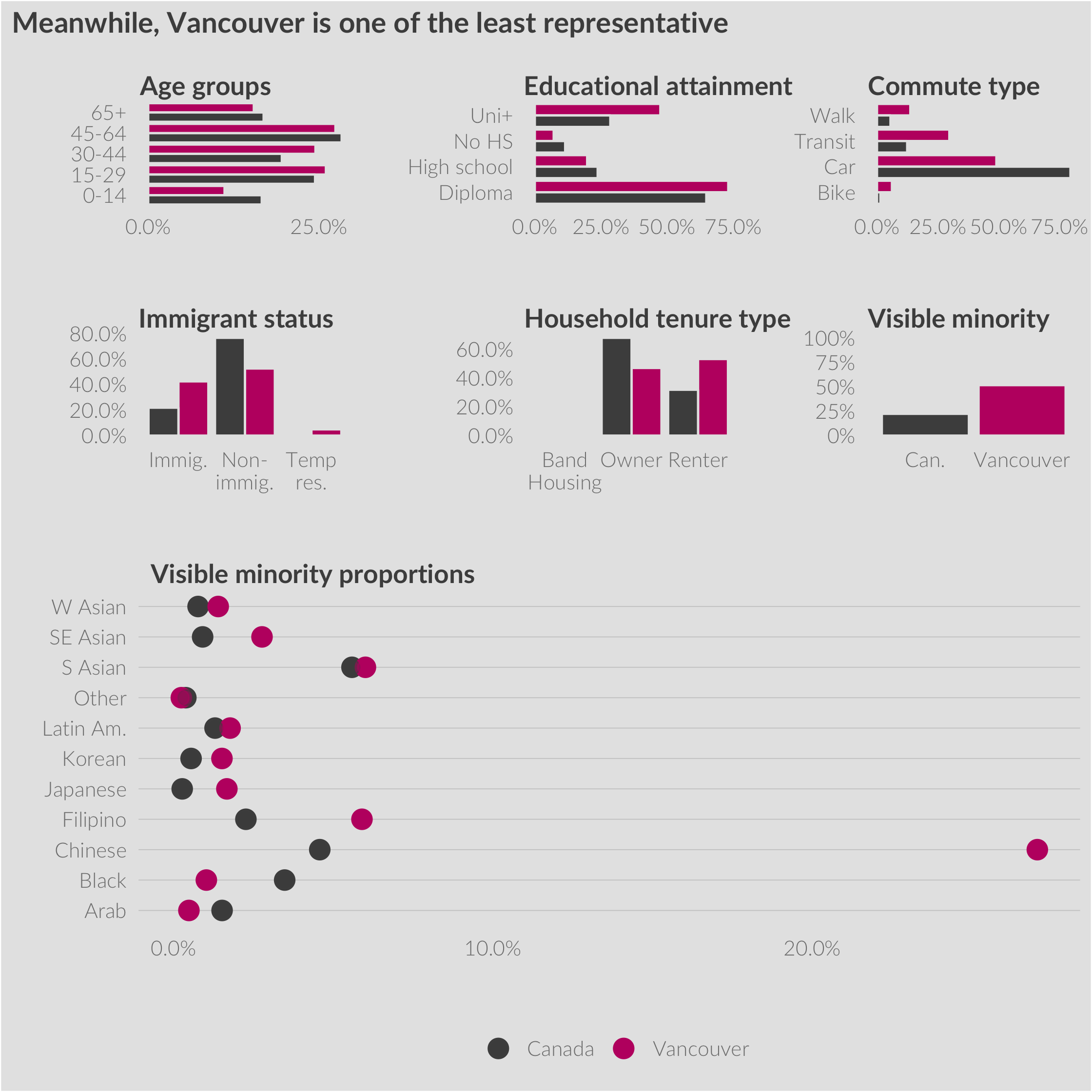 Canada’s major population centres: the GTA, Montreal, and the Lower Mainland all tend to have a higher educational attainment, different commuting patterns, more renters, and much more visible diversity. Because these few metropolitan regions account for so much of the national population, they will skew the national rates to reflect these differences.
Of the most similar cities on the list, the first 9 municipalities all have larger populations. The smaller towns with high similarity scores, View Royal, BC and L’Île-Perrot, QC are extended suburbs of Victoria and Montreal, respectively. If the objective of something like this is to find the definitive small Canadian town with the demographic mix that best represents the country and is not within the immediate geographic influence of a larger metropolitan area, you have to wait to the 24-th ranked city on the list, Brandon, MB. This is not unexpected as any Canadian average will be significantly weighted by larger metropolitan areas that tend to be more educated and more diverse than smaller cities outside of core metro areas.
| Municipality | Population | Similarity Score |
|---|---|---|
| Châteauguay | 47,906 | 82.8 |
| Brandon | 48,859 | 81.6 |
| Vaudreuil-Dorion | 38,117 | 81.4 |
| Whitehorse | 25,085 | 81.1 |
| Langford | 35,342 | 80.7 |
| Note: | ||
| Source: Statistics Canada Census 2016 |
Find your city
You can scroll the full table below which has the similarity scores for all Canadian municipalities and municipality-like regions with populations above 10,000.
| Municipality | Population | Similarity Score |
|---|---|---|
| Hamilton (C) | 536,917 | 91.6 |
| Guelph | 131,794 | 89.1 |
| London | 383,822 | 88.0 |
| Winnipeg | 705,244 | 87.4 |
| Kitchener | 233,222 | 86.5 |
| Saskatoon | 246,376 | 86.3 |
| Laval | 422,993 | 86.0 |
| Saanich | 114,148 | 85.9 |
| Regina | 215,106 | 85.7 |
| View Royal | 10,408 | 85.5 |
| L’Île-Perrot | 10,756 | 84.1 |
| Pitt Meadows | 18,573 | 83.9 |
| St. Catharines | 133,113 | 83.4 |
| Windsor | 217,188 | 83.0 |
| Oshawa | 159,458 | 82.8 |
| Châteauguay | 47,906 | 82.8 |
| Gatineau | 276,245 | 82.4 |
| Dorval | 18,980 | 82.2 |
| Kelowna | 127,380 | 82.2 |
| Newmarket | 84,224 | 82.0 |
| Nanaimo | 90,504 | 82.0 |
| Burlington | 183,314 | 81.9 |
| Squamish | 19,512 | 81.9 |
| Brandon | 48,859 | 81.6 |
| Lethbridge | 92,729 | 81.5 |
| Vaudreuil-Dorion | 38,117 | 81.4 |
| Edmonton | 932,546 | 81.2 |
| Cambridge | 129,920 | 81.2 |
| Whitehorse | 25,085 | 81.1 |
| Red Deer | 100,418 | 80.9 |
| Kingston | 123,798 | 80.7 |
| Langford | 35,342 | 80.7 |
| Niagara Falls | 88,071 | 80.5 |
| Port Coquitlam | 58,612 | 80.4 |
| Barrie | 141,434 | 80.1 |
| Whitby | 128,377 | 80.0 |
| Maple Ridge | 82,256 | 79.8 |
| Langley (CY) | 25,888 | 79.7 |
| La Prairie | 24,110 | 79.5 |
| White Rock | 19,952 | 79.4 |
| Ottawa | 934,243 | 79.4 |
| Halifax | 403,131 | 79.4 |
| Calgary | 1,239,220 | 79.1 |
| Longueuil | 239,700 | 78.9 |
| Terrace | 11,643 | 78.8 |
| Colwood | 16,859 | 78.3 |
| Pointe-Claire | 31,380 | 78.2 |
| Kamloops | 90,280 | 78.1 |
| Langley (DM) | 117,285 | 78.1 |
| Waterloo | 104,986 | 77.7 |
| Sarnia | 71,594 | 77.6 |
| Peterborough | 81,032 | 77.4 |
| Brantford | 97,496 | 77.1 |
| Delta | 102,238 | 77.0 |
| Courtenay | 25,599 | 77.0 |
| Canmore | 13,992 | 77.0 |
| Deux-Montagnes | 17,496 | 76.9 |
| Thorold | 18,801 | 76.9 |
| Thunder Bay | 107,909 | 76.9 |
| Port Moody | 33,551 | 76.9 |
| North Battleford | 14,315 | 76.8 |
| Central Saanich | 16,814 | 76.7 |
| Stratford | 31,465 | 76.7 |
| Prince George | 74,003 | 76.7 |
| Steinbach | 15,829 | 76.4 |
| Boisbriand | 26,884 | 76.4 |
| Bradford West Gwillimbury | 35,325 | 76.3 |
| Moncton | 71,889 | 76.1 |
| Lloydminster (Part) (CY) | 19,645 | 76.1 |
| Fredericton | 58,220 | 76.1 |
| Collingwood | 21,793 | 75.9 |
| North Cowichan | 29,676 | 75.9 |
| Repentigny | 84,285 | 75.9 |
| Saltspring Island | 10,557 | 75.8 |
| Penticton | 33,761 | 75.8 |
| Camrose | 18,742 | 75.7 |
| St. John’s | 108,860 | 75.7 |
| Sechelt | 10,216 | 75.7 |
| Vernon | 40,116 | 75.6 |
| Saint-Eustache | 44,008 | 75.4 |
| Lacombe | 13,057 | 75.4 |
| High River | 13,584 | 75.3 |
| Yellowknife | 19,569 | 75.1 |
| Sooke | 13,001 | 75.0 |
| Chilliwack | 83,788 | 75.0 |
| Comox | 14,028 | 74.8 |
| Sault Ste. Marie | 73,368 | 74.8 |
| Terrebonne | 111,575 | 74.7 |
| Orangeville | 28,900 | 74.7 |
| Cold Lake | 14,961 | 74.7 |
| Aurora | 55,445 | 74.7 |
| Prince Rupert | 12,220 | 74.6 |
| King | 24,512 | 74.6 |
| Sainte-Catherine | 17,047 | 74.6 |
| Saint-Constant | 27,359 | 74.5 |
| Greater Sudbury | 161,531 | 74.5 |
| Wood Buffalo | 71,589 | 74.5 |
| Cobourg | 19,440 | 74.5 |
| Yorkton | 16,343 | 74.5 |
| Belleville | 50,716 | 74.4 |
| Swift Current | 16,604 | 74.4 |
| Weyburn | 10,870 | 74.3 |
| Pincourt | 14,558 | 74.3 |
| Campbell River | 32,588 | 74.3 |
| Cranbrook | 20,047 | 74.2 |
| Mission | 38,833 | 74.2 |
| Abbotsford | 141,397 | 74.1 |
| Leduc | 29,993 | 74.1 |
| North Vancouver (DM) | 85,935 | 74.0 |
| Medicine Hat | 63,260 | 74.0 |
| Prince Albert | 35,926 | 73.9 |
| Carleton Place | 10,644 | 73.9 |
| Lake Country | 12,922 | 73.9 |
| Grande Prairie | 63,166 | 73.9 |
| St. Albert | 65,589 | 73.9 |
| Halton Hills | 61,161 | 73.9 |
| Wetaskiwin | 12,655 | 73.9 |
| Moose Jaw | 33,890 | 73.8 |
| Welland | 52,293 | 73.8 |
| Orillia | 31,166 | 73.8 |
| North Bay | 51,553 | 73.7 |
| Estevan | 11,483 | 73.7 |
| Kincardine | 11,389 | 73.6 |
| Saugeen Shores | 13,715 | 73.5 |
| Charlottetown | 36,094 | 73.5 |
| Fort St. John | 20,155 | 73.4 |
| Dawson Creek | 12,178 | 73.4 |
| Lloydminster (Part) (CY) | 11,765 | 73.4 |
| Chambly | 29,120 | 73.3 |
| Salmon Arm | 17,706 | 73.3 |
| Fort Saskatchewan | 24,149 | 73.2 |
| Okotoks | 28,881 | 73.1 |
| Dollard-Des Ormeaux | 48,899 | 73.1 |
| Woodstock | 40,902 | 73.0 |
| Airdrie | 61,581 | 73.0 |
| Powell River | 13,157 | 72.9 |
| Nelson | 10,572 | 72.9 |
| West Kelowna | 32,655 | 72.8 |
| Saint John | 67,575 | 72.8 |
| St. Thomas | 38,909 | 72.8 |
| East Gwillimbury | 23,991 | 72.7 |
| Grimsby | 27,314 | 72.7 |
| Port Hope | 16,753 | 72.7 |
| Blainville | 56,863 | 72.7 |
| Sherbrooke | 161,323 | 72.6 |
| Québec | 531,902 | 72.6 |
| Sidney | 11,672 | 72.5 |
| Dieppe | 25,384 | 72.4 |
| Caledon | 66,502 | 72.2 |
| Strathmore | 13,756 | 72.2 |
| Fort Erie | 30,710 | 72.2 |
| Uxbridge | 21,176 | 72.2 |
| Stony Plain | 17,189 | 72.1 |
| Port Alberni | 17,678 | 72.1 |
| Williams Lake | 10,753 | 72.1 |
| Midland | 16,864 | 72.1 |
| Strathroy-Caradoc | 20,867 | 72.0 |
| Brockville | 21,346 | 72.0 |
| Cochrane | 25,853 | 71.9 |
| Chatham-Kent | 101,647 | 71.9 |
| Centre Wellington | 28,191 | 71.9 |
| Spruce Grove | 34,066 | 71.8 |
| Beloeil | 22,458 | 71.8 |
| Woolwich | 25,006 | 71.8 |
| Saint-Jean-sur-Richelieu | 95,114 | 71.7 |
| Kenora | 15,096 | 71.7 |
| Esquimalt | 17,655 | 71.7 |
| Sainte-Adèle | 12,919 | 71.7 |
| L’Ancienne-Lorette | 16,543 | 71.6 |
| Kings, Subd. B | 11,858 | 71.6 |
| Summerland | 11,615 | 71.6 |
| Tecumseh | 23,229 | 71.6 |
| New Tecumseth | 34,242 | 71.5 |
| Whistler | 11,854 | 71.5 |
| Clarington | 92,013 | 71.5 |
| Timmins | 41,788 | 71.4 |
| Portage la Prairie | 13,304 | 71.3 |
| Owen Sound | 21,341 | 71.2 |
| L’Assomption | 22,429 | 71.2 |
| Mercier | 13,115 | 71.2 |
| Mascouche | 46,692 | 71.2 |
| Lévis | 143,414 | 71.1 |
| Riverview | 19,667 | 71.1 |
| Lincoln | 23,787 | 71.1 |
| Whitchurch-Stouffville | 45,837 | 71.0 |
| Georgina | 45,418 | 71.0 |
| Meaford | 10,991 | 71.0 |
| Saint-Sauveur | 10,231 | 70.8 |
| Pickering | 91,771 | 70.8 |
| Lethbridge County | 10,353 | 70.7 |
| Varennes | 21,257 | 70.7 |
| Rouyn-Noranda | 42,334 | 70.7 |
| Gander | 11,688 | 70.6 |
| Port Colborne | 18,306 | 70.6 |
| Corner Brook | 19,806 | 70.6 |
| Parksville | 12,514 | 70.6 |
| Clarence-Rockland | 24,512 | 70.6 |
| Edmundston | 16,580 | 70.6 |
| Sainte-Marie | 13,565 | 70.6 |
| Candiac | 21,047 | 70.6 |
| Strathcona County | 98,044 | 70.6 |
| Tillsonburg | 15,872 | 70.5 |
| Niagara-on-the-Lake | 17,511 | 70.4 |
| Sainte-Thérèse | 25,989 | 70.4 |
| Marieville | 10,725 | 70.3 |
| Cape Breton | 94,285 | 70.3 |
| Kingsville | 21,552 | 70.3 |
| Whitecourt | 10,204 | 70.2 |
| Mount Pearl | 22,957 | 70.2 |
| Mississippi Mills | 13,163 | 70.2 |
| Trois-Rivières | 134,413 | 70.2 |
| Leamington | 27,595 | 70.2 |
| Rimouski | 48,664 | 70.2 |
| Bracebridge | 16,010 | 70.1 |
| Rocky View County | 39,407 | 70.1 |
| Mirabel | 50,513 | 70.1 |
| Brossard | 85,721 | 70.1 |
| Victoriaville | 46,130 | 70.0 |
| Oakville | 193,832 | 70.0 |
| Huntsville | 19,816 | 70.0 |
| Norfolk County | 64,044 | 70.0 |
| Loyalist | 16,971 | 70.0 |
| Beaumont | 17,396 | 70.0 |
| Wilmot | 20,545 | 70.0 |
| Brooks | 14,451 | 69.9 |
| Miramichi | 17,537 | 69.9 |
| Sept-Îles | 25,400 | 69.8 |
| Quinte West | 43,577 | 69.8 |
| Petawawa | 17,187 | 69.8 |
| Val-d’Or | 32,491 | 69.8 |
| Grand Falls-Windsor | 14,171 | 69.8 |
| Russell | 16,520 | 69.8 |
| South Huron | 10,096 | 69.8 |
| Sylvan Lake | 14,816 | 69.8 |
| Scugog | 21,617 | 69.8 |
| North Saanich | 11,249 | 69.8 |
| Sainte-Julie | 29,881 | 69.7 |
| Essa | 21,083 | 69.7 |
| Greater Napanee | 15,892 | 69.7 |
| New Westminster | 70,996 | 69.7 |
| Kings, Subd. A | 22,234 | 69.7 |
| Ingersoll | 12,757 | 69.7 |
| Magog | 26,669 | 69.6 |
| Rawdon | 11,057 | 69.5 |
| Colchester, Subd. B | 19,534 | 69.5 |
| Foothills No. 31 | 22,766 | 69.5 |
| Coldstream | 10,648 | 69.4 |
| Rosemère | 13,958 | 69.4 |
| Rothesay | 11,659 | 69.4 |
| Baie-Comeau | 21,536 | 69.4 |
| Gravenhurst | 12,311 | 69.4 |
| Prince Edward County | 24,735 | 69.4 |
| North Dundas | 11,278 | 69.4 |
| Granby | 66,222 | 69.4 |
| Amherstburg | 21,936 | 69.3 |
| Selkirk | 10,278 | 69.3 |
| Erin | 11,439 | 69.3 |
| Brant | 36,707 | 69.3 |
| Innisfil | 36,566 | 69.3 |
| Pembroke | 13,882 | 69.3 |
| Saint-Hyacinthe | 55,648 | 69.3 |
| Mont-Saint-Hilaire | 18,585 | 69.3 |
| North Perth | 13,130 | 69.2 |
| Saguenay | 145,949 | 69.2 |
| Guelph/Eramosa | 12,854 | 69.2 |
| Beauharnois | 12,884 | 69.2 |
| Summerside | 14,829 | 69.2 |
| North Dumfries | 10,215 | 69.1 |
| Amos | 12,823 | 69.1 |
| Chestermere | 19,887 | 69.1 |
| Saint-Jérôme | 74,346 | 69.0 |
| Saint-Georges | 32,513 | 69.0 |
| Drummondville | 75,423 | 68.9 |
| Pelham | 17,110 | 68.8 |
| Bathurst | 11,897 | 68.8 |
| North Glengarry | 10,109 | 68.8 |
| Saint-Félicien | 10,238 | 68.8 |
| West Nipissing | 14,364 | 68.7 |
| Brighton | 11,844 | 68.7 |
| The Nation | 12,808 | 68.7 |
| Matane | 14,311 | 68.7 |
| Alma | 30,776 | 68.7 |
| Sainte-Agathe-des-Monts | 10,223 | 68.7 |
| LaSalle | 30,180 | 68.6 |
| Brock | 11,642 | 68.6 |
| Sorel-Tracy | 34,755 | 68.6 |
| Bécancour | 13,031 | 68.5 |
| North Vancouver (CY) | 52,898 | 68.4 |
| Lambton Shores | 10,631 | 68.4 |
| Sainte-Anne-des-Plaines | 14,421 | 68.4 |
| Cornwall | 46,589 | 68.4 |
| North Grenville | 16,451 | 68.4 |
| Trent Hills | 12,900 | 68.3 |
| Haldimand County | 45,608 | 68.3 |
| Saint-Basile-le-Grand | 17,059 | 68.3 |
| Winkler | 12,591 | 68.2 |
| Rivière-du-Loup | 19,507 | 68.2 |
| Sturgeon County | 20,495 | 68.2 |
| Roberval | 10,046 | 68.2 |
| Norwich | 11,001 | 68.1 |
| Lakeshore | 36,611 | 68.1 |
| Essex | 20,427 | 68.0 |
| Wellington North | 11,914 | 68.0 |
| Gaspé | 14,568 | 68.0 |
| Sainte-Marthe-sur-le-Lac | 18,074 | 67.9 |
| Springwater | 19,059 | 67.9 |
| South Glengarry | 13,150 | 67.8 |
| Notre-Dame-de-l’Île-Perrot | 10,654 | 67.8 |
| La Tuque | 11,001 | 67.8 |
| Kawartha Lakes | 75,423 | 67.8 |
| Dolbeau-Mistassini | 14,250 | 67.7 |
| Elliot Lake | 10,741 | 67.7 |
| Montmagny | 11,255 | 67.7 |
| Selwyn | 17,060 | 67.6 |
| Clearview | 14,151 | 67.6 |
| Central Elgin | 12,607 | 67.6 |
| Thetford Mines | 25,403 | 67.6 |
| Middlesex Centre | 17,262 | 67.6 |
| Colchester, Subd. C | 13,098 | 67.6 |
| South Dundas | 10,833 | 67.6 |
| East Hants | 22,453 | 67.6 |
| Lacombe County | 10,343 | 67.5 |
| St. Clair | 14,086 | 67.5 |
| Oak Bay | 18,094 | 67.5 |
| Thames Centre | 13,191 | 67.4 |
| Saint-Lazare | 19,889 | 67.4 |
| Mont-Laurier | 14,116 | 67.4 |
| West Grey | 12,518 | 67.4 |
| Milton | 110,128 | 67.3 |
| Boucherville | 41,671 | 67.3 |
| Truro | 12,261 | 67.3 |
| Chester | 10,310 | 67.3 |
| Wasaga Beach | 20,675 | 67.3 |
| Conception Bay South | 26,199 | 67.2 |
| Shawinigan | 49,349 | 67.2 |
| Salaberry-de-Valleyfield | 40,745 | 67.2 |
| Leduc County | 13,780 | 67.2 |
| Coquitlam | 139,284 | 67.1 |
| Saint-Bruno-de-Montarville | 26,394 | 67.1 |
| Saint-Charles-Borromée | 13,791 | 67.0 |
| West Lincoln | 14,500 | 67.0 |
| Mountain View County | 13,074 | 67.0 |
| Prévost | 13,002 | 66.7 |
| Cowansville | 13,656 | 66.6 |
| West Hants | 15,368 | 66.6 |
| Saint-Amable | 12,167 | 66.5 |
| Paradise | 21,389 | 66.5 |
| Saint-Raymond | 10,221 | 66.5 |
| Lavaltrie | 13,657 | 66.5 |
| Adjala-Tosorontio | 10,975 | 66.3 |
| Tiny | 11,787 | 66.3 |
| Vaughan | 306,233 | 66.3 |
| Val-des-Monts | 11,582 | 66.3 |
| Kirkland | 20,151 | 66.2 |
| Severn | 13,477 | 66.2 |
| Queens | 10,307 | 66.1 |
| Warman | 11,020 | 66.1 |
| Sainte-Sophie | 15,690 | 66.0 |
| Les Îles-de-la-Madeleine | 12,010 | 66.0 |
| Taché | 11,568 | 65.9 |
| Wetaskiwin County No. 10 | 11,181 | 65.8 |
| Red Deer County | 19,541 | 65.8 |
| Cantley | 10,699 | 65.8 |
| South Stormont | 13,110 | 65.8 |
| Oro-Medonte | 21,036 | 65.6 |
| Saint-Lin–Laurentides | 20,786 | 65.6 |
| Saint-Lambert | 21,861 | 65.5 |
| Perth East | 12,261 | 65.5 |
| Yellowhead County | 10,995 | 65.5 |
| Parkland County | 32,097 | 65.5 |
| Quispamsis | 18,245 | 65.4 |
| Rideau Lakes | 10,326 | 65.3 |
| Georgian Bluffs | 10,479 | 65.2 |
| South Frontenac | 18,646 | 65.2 |
| Tay | 10,033 | 65.1 |
| Hamilton (TP) | 10,942 | 65.1 |
| Saint-Colomban | 16,019 | 65.0 |
| Joliette | 20,484 | 64.9 |
| Ajax | 119,677 | 64.9 |
| Lunenburg | 24,863 | 64.7 |
| Hanover | 15,733 | 64.4 |
| Saint-Augustin-de-Desmaures | 18,820 | 64.4 |
| Beaconsfield | 19,324 | 64.3 |
| Springfield | 15,342 | 64.3 |
| St. Andrews | 11,913 | 64.2 |
| Clearwater County | 11,947 | 64.2 |
| Grande Prairie County No. 1 | 22,303 | 64.2 |
| Surrey | 517,887 | 64.1 |
| West Vancouver | 42,473 | 64.1 |
| Lachute | 12,862 | 63.9 |
| St. Clements | 10,876 | 63.9 |
| Wellesley | 11,260 | 63.9 |
| Côte-Saint-Luc | 32,448 | 63.9 |
| Bonnyville No. 87 | 13,575 | 63.8 |
| Hawkesbury | 10,263 | 63.5 |
| Tracadie | 16,114 | 63.5 |
| Lac Ste. Anne County | 10,899 | 63.5 |
| Victoria | 85,792 | 63.1 |
| Mapleton | 10,527 | 63.0 |
| Mont-Royal | 20,276 | 63.0 |
| Mississauga | 721,599 | 61.6 |
| Montréal | 1,704,694 | 60.5 |
| Toronto | 2,731,571 | 59.6 |
| Westmount | 20,312 | 59.2 |
| Vancouver | 631,486 | 58.3 |
| Burnaby | 232,755 | 57.9 |
| Richmond Hill | 195,022 | 56.6 |
| Mackenzie County | 11,171 | 55.5 |
| Brampton | 593,638 | 55.3 |
| Markham | 328,966 | 51.9 |
| Richmond | 198,309 | 51.7 |
| Greater Vancouver A | 16,133 | 46.6 |
| Note: | ||
| Source: Statistics Canada Census 2016. |
Mirror images - a detour
There are many dimensions we can use to measure similarity across cities and, by extension, many assumptions to consider when doing so. The similarity numbers used here reflect assumptions about both which dimensions should be included or excluded and the method through which we evaluate similarity. A different selection of variables or dimensions would likely lead to a different result. Even the way that variables are aggregated here could affect the results. This is all to say that this post is not trying to be a definitive study of city similarity and that it is affected by the choices made by the author in terms of what to measure–and how. This caveat applies to both this post and to the source FiveThirtyEight post. New Haven is the most “normal” city in America (based on that article’s author’s choice of relevant variables and methodology). It might still be the most “normal” given a different set of input variables, but it might also not be.
Just as using a different set of variables could lead to different results, a different distance measure for similarity or a different measurement methodology could lead to different results as well. There are many different ways to measure something like this.
One approach to something like this is to use algorithms that map high-dimensional data into lower dimensional space to visually display similarity between many high-dimensional objects at the same time. In an older post, I wrote about identifying clusters of Canadian cities based on similarity in either visible minority group, education, or occupation. That post used an application of the t-SNE algorithm for visualizing closeness for high-dimensional data. The upside of that approach versus something like the geometric similarity index used in this post is that it shows relationships between all selected cities instead of one city at a time.
Something similar can be done with the multi-dimensional data used in calculating the similarity indices above. The unifold manifold approximation and projection (UMAP) algorithm is another method that is increasingly used in lieu of t-SNE for dimensional reduction and visualization in lower dimensional space. UMAP has some advantages over t-SNE in that it tends to be computationally faster and, more importantly for us, tends to do a better job in preserving global structure in lower-dimensional embeddings. Typically in t-SNE embeddings objects close together are similar across their many dimensions, but objects far from one another are not necessarily dissimilar, which can be counter-intuitive for someone looking at the resulting visualization.
The below visualization shows a UMAP embedding using the same variables as in the similarity index for all Census subdivisions with populations above 100,000. In this visualization, the national demographic and characteristic mix is embedded in the middle and the CSDs with the most similar mixes should be located closest to that point. Notably, this approach produces some differences in results. Hamilton, while still very similar, is no longer the most “normal” CSD. That distinction falls to Windsor, Ontario, with Saanich, BC also in close proximity. There is a pretty good overlap in the cities identified by this approach and the similarity indices above which is a good sign that we can consider that group of cities as representative of a “normal” Canada–if at least for this combination of demographic and characteristic variables. UMAP embeddings have an element of randomness to them and the exact layout will be different every time it is generated, but there should be consistency in the approximate placement of individual points if there is an actual structure to the data.
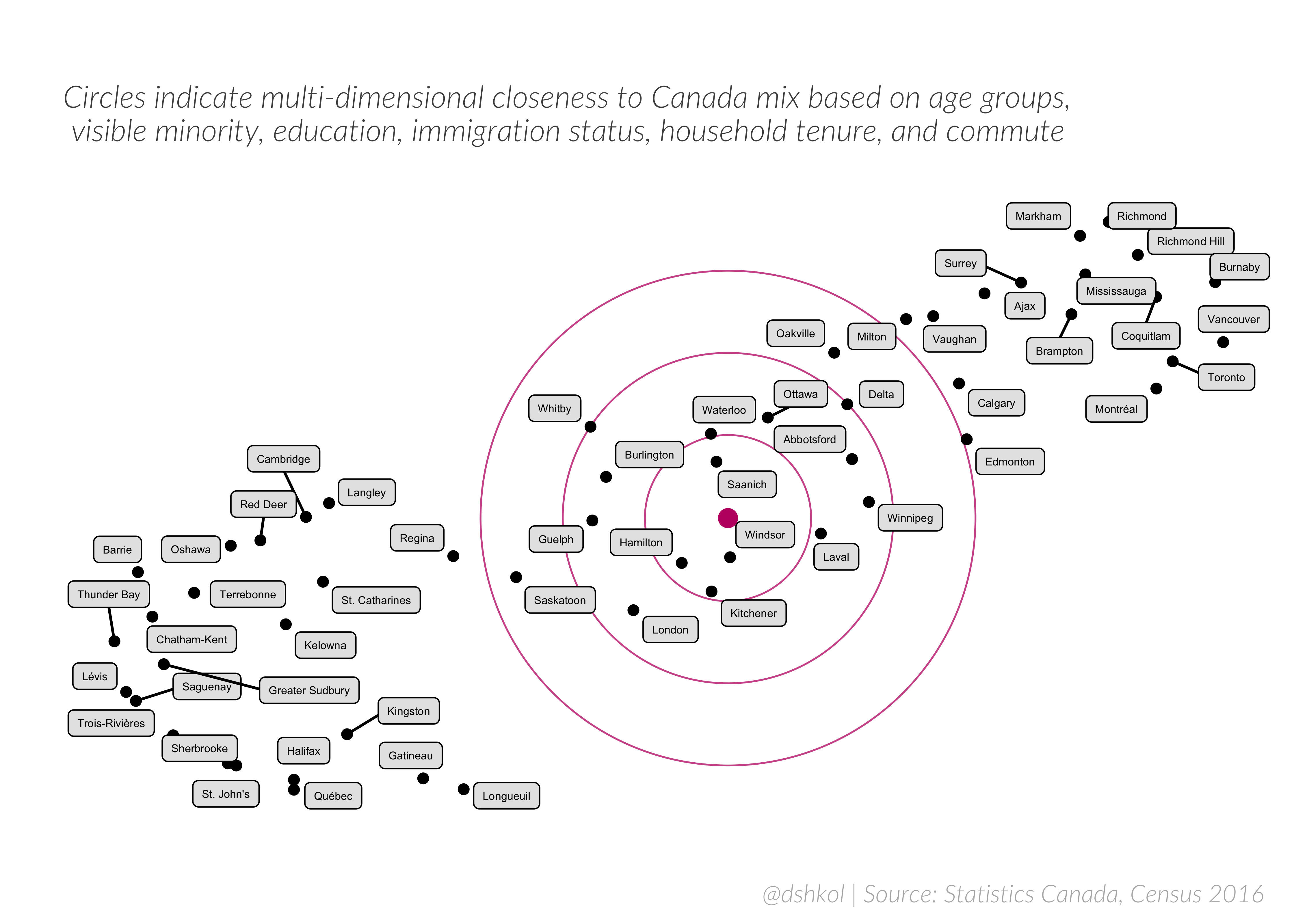 The advantage of this approach is it shows both the similarity and dissimilarity of these CSDs to the national mix, but it also can be interpreted to show similarity and dissimilarity of these CSDs from one another. Richmond and Richmond Hill have high similarity to another one, as do Sherbrooke and St. John’s, but the same visual layout shows that Sherbrooke and Richmond Hill have very different compositions from one another.
Show us the guts
The code for getting Census data, transforming it, and calculating the similarity scores is below. The code for this entire page is, as always, view-able on Github. The UMAP visualization takes advantage of the excellent umap R package.
# Load required packages
library(cancensus)
library(dplyr)
library(tidyr)

# Generate list of Census Subdivisions in Canada with pop >= 100000
csdlist <- list_census_regions("CA16") %>%
  filter(pop >= 10000, level == "CSD") %>%
  as_census_region_list()

# Get region code for Canada-wide region
national_region <- list_census_regions("CA16") %>% filter(level == "C") %>% as_census_region_list()

# Convenience function to tidy up CSD names
clean_names2 <- function (dfr) {
  dfr <- dfr %>% mutate(`Region Name` = as.character(`Region Name`))
  replacement <- dfr %>% mutate(`Region Name` = gsub(" \\(.*\\)",
                                                     "", `Region Name`)) %>% pull(`Region Name`)
  duplicated_rows <- c(which(duplicated(replacement, fromLast = TRUE)),
                       which(duplicated(replacement, fromLast = FALSE)))
  replacement[duplicated_rows] <- dfr$`Region Name`[duplicated_rows]
  dfr$`Region Name` <- factor(replacement)
  dfr
}

# Identify appropriate vector codes
# 0-14, 15-29, 30-44, 45-64, 65+
age_vectors <- c("v_CA16_1", "v_CA16_4", "v_CA16_64", "v_CA16_82","v_CA16_100",
          "v_CA16_118","v_CA16_136", "v_CA16_154","v_CA16_172","v_CA16_190",
          "v_CA16_208","v_CA16_226","v_CA16_244")

# Visible minorities vectors
parent_vector <- "v_CA16_3954"
minorities <- list_census_vectors("CA16") %>%
  filter(vector == "v_CA16_3954") %>%
  child_census_vectors(leaves_only = TRUE) %>%
  pull(vector)
minority_vectors <- c(parent_vector, minorities)

# Education vectors - uses only data for population aged 25 and over.
# no diploma, high-school, post-secondary certificate, university diploma or higher
educ_vectors <- c("v_CA16_5096", "v_CA16_5099", "v_CA16_5102", "v_CA16_5105", "v_CA16_5123")

# Immigration status vectors
imm_vectors <- c("v_CA16_3405","v_CA16_3408","v_CA16_3411","v_CA16_3435")

# Tenure vectors
ten_vectors <- c("v_CA16_4836","v_CA16_4837","v_CA16_4838","v_CA16_4839")

# Commute vectors
com_vectors <- c("v_CA16_5792","v_CA16_5795","v_CA16_5798","v_CA16_5801",
                 "v_CA16_5804","v_CA16_5807")

# Mobility vectors
#mob_vectors <- c("v_CA16_6692", "v_CA16_6707","v_CA16_6716")

# Coerce all vectors requested together
demo_vectors <- c(age_vectors, minority_vectors, educ_vectors, imm_vectors, ten_vectors, com_vectors)

# Download census data for national level
national <- get_census("CA16", level = "C", regions = national_region, vectors = demo_vectors, labels = "short")

# Group vectors where appropriate and calculate proportions
national_demo <- national %>%
  mutate(age_014 = v_CA16_4/v_CA16_1,
         age_1529 = (v_CA16_64 + v_CA16_64 + v_CA16_82 + v_CA16_100)/v_CA16_1,
         age_3044 = (v_CA16_118 + v_CA16_136 + v_CA16_154)/v_CA16_1,
         age_4564 = (v_CA16_172 + v_CA16_190 + v_CA16_208 + v_CA16_226)/v_CA16_1,
         age_65p = v_CA16_244/v_CA16_1,
         min_white = v_CA16_3996/v_CA16_3954,
         min_sasian = v_CA16_3960/v_CA16_3954,
         min_chinese = v_CA16_3963/v_CA16_3954,
         min_black = v_CA16_3966/v_CA16_3954,
         min_filipino = v_CA16_3969/v_CA16_3954,
         min_latinam = v_CA16_3972/v_CA16_3954,
         min_arab = v_CA16_3975/v_CA16_3954,
         min_seasian = v_CA16_3978/v_CA16_3954,
         min_wasian = v_CA16_3981/v_CA16_3954,
         min_korean = v_CA16_3984/v_CA16_3954,
         min_japanese = v_CA16_3987/v_CA16_3954,
         min_oth = v_CA16_3990/v_CA16_3954,
         educ_nohs = v_CA16_5099/v_CA16_5096,
         educ_hs = v_CA16_5102/v_CA16_5096,
         educ_dip = v_CA16_5105/v_CA16_5096,
         educ_uni = v_CA16_5123/v_CA16_5096,
         imm_nat = v_CA16_3408/v_CA16_3405,
         imm_imm = v_CA16_3411/v_CA16_3405,
         imm_non = v_CA16_3435/v_CA16_3405,
         ten_own = v_CA16_4837/v_CA16_4836,
         ten_rent = v_CA16_4838/v_CA16_4836,
         ten_band = v_CA16_4839/v_CA16_4836,
         com_car = (v_CA16_5795 + v_CA16_5798)/v_CA16_5792,
         com_trans = v_CA16_5801/v_CA16_5792,
         com_walk = v_CA16_5804/v_CA16_5792,
         com_bike = v_CA16_5807/v_CA16_5792) %>%
  select(GeoUID, `Region Name`, pop = Population, starts_with("age"), starts_with("min"), starts_with("educ"),
         starts_with("imm"), starts_with("ten"), starts_with("com"))

# Get demographic vectors for all selected csds
csds <- get_census("CA16", level = "CSD", regions = csdlist, vectors = demo_vectors, labels = "short")

# adjust into groups and calculate proportions - same as above.
csds <- csds %>%
  mutate(age_014 = v_CA16_4/v_CA16_1,
         age_1529 = (v_CA16_64 + v_CA16_64 + v_CA16_82 + v_CA16_100)/v_CA16_1,
         age_3044 = (v_CA16_118 + v_CA16_136 + v_CA16_154)/v_CA16_1,
         age_4564 = (v_CA16_172 + v_CA16_190 + v_CA16_208 + v_CA16_226)/v_CA16_1,
         age_65p = v_CA16_244/v_CA16_1,
         min_white = v_CA16_3996/v_CA16_3954,
         min_sasian = v_CA16_3960/v_CA16_3954,
         min_chinese = v_CA16_3963/v_CA16_3954,
         min_black = v_CA16_3966/v_CA16_3954,
         min_filipino = v_CA16_3969/v_CA16_3954,
         min_latinam = v_CA16_3972/v_CA16_3954,
         min_arab = v_CA16_3975/v_CA16_3954,
         min_seasian = v_CA16_3978/v_CA16_3954,
         min_wasian = v_CA16_3981/v_CA16_3954,
         min_korean = v_CA16_3984/v_CA16_3954,
         min_japanese = v_CA16_3987/v_CA16_3954,
         min_oth = v_CA16_3990/v_CA16_3954,
         educ_nohs = v_CA16_5099/v_CA16_5096,
         educ_hs = v_CA16_5102/v_CA16_5096,
         educ_dip = v_CA16_5105/v_CA16_5096,
         educ_uni = v_CA16_5123/v_CA16_5096,
         imm_nat = v_CA16_3408/v_CA16_3405,
         imm_imm = v_CA16_3411/v_CA16_3405,
         imm_non = v_CA16_3435/v_CA16_3405,
         ten_own = v_CA16_4837/v_CA16_4836,
         ten_rent = v_CA16_4838/v_CA16_4836,
         ten_band = v_CA16_4839/v_CA16_4836,
         com_car = (v_CA16_5795 + v_CA16_5798)/v_CA16_5792,
         com_trans = v_CA16_5801/v_CA16_5792,
         com_walk = v_CA16_5804/v_CA16_5792,
         com_bike = v_CA16_5807/v_CA16_5792) %>%
  select(GeoUID, `Region Name`, pop = Population, starts_with("age"), starts_with("min"), starts_with("educ"),
         starts_with("imm"), starts_with("ten"), starts_with("com"))

# Finally, calculate pairwise dissimilarity between each CSD and the national rates using a Euclidian distance measurement and then calculate an index value for how closely similar or not CSDs are to national rates.
diss <- bind_rows(national_demo, csds) %>%
  mutate_at(vars(age_014:com_bike), funs((.- first(.))^2)) %>%
  tidyr::gather(vars, values, age_014:com_bike) %>%
  group_by(`Region Name`, pop) %>%
  summarise(index = sqrt(sum(values))) %>%
  mutate(sim = (1/(1+index)*100)) %>%
  ungroup() %>%
  filter(`Region Name` != "Canada") %>%
  clean_names2()